Streak Camera : Error corrections
Streak camera sensitivity along the time axis
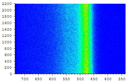
The streak camera was used to measure cw (continuous)light, in this case a white LED.
Since this light has no time dependence, it should have the same height, at all timevalues.
The following data was measured with Synchroscan timebase 4 (30000×56 ms exposures, monochromater slit 10 micron, streak camera slit 20 micron).
[ file: : D:\Lab documentation\5117.-109 Streak camera\Anomaly correction measurements\2016-02-25 LED TB1-4\timebase4.txt.
Download raw data: led_tb1-4.zip ]
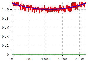
If this data is integrated over all frequencies (x-axis), is normalized so the center has height 1, and is displayed as a function of time (red, in ps):
[ file: D:\Lab documentation\5117.-109 Streak camera\Anomaly correction measurements\2016-02-25 LED TB1-4\Analysis\timebase4 fit.txt ]
It is not a straight line, as it should be, but somewhat quadratic. The blue line is a 2nd degree polynomial fit. A 4th degree is even slightly better.
Possibly, the time sweep is not linear : maybe it is slower at the beginning and the end, and would then accumulate more photons.
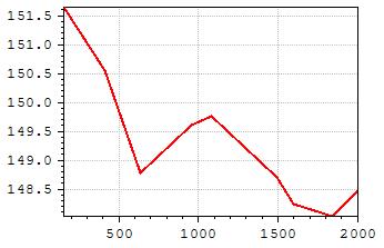
To test this, a series of exposures was made with the light of the Mira, going through 2 (roughly) 50% reflecting, parallel mirrors, separated by 22.2 (+/- 0.1) mm. This produces a pulse, followed by a second pulse (about 5 times smaller), delayed by 148 ps (and even an entire weaker and weaker pulse train). By using different delay settings of the streak camera, this pulse pair was measured at 9 different positions on the time axis. At each position, the pulses where fitted, and the time delay between the 2 was determined. If the time-axis of the streak camera is non-linear, these time-delays should appear different at different position on the time axis.
[file: D:\Lab documentation\5117.-109 Streak camera\Anomaly correction measurements\2016-03-07 Linearity Timebase 4\Analysis\DeltaT vs T.txt]
The y-values are the time difference between the 2 pulses. The x-values are the center-time of the 2 pulses. There is some difference between the delay of the time pulses. But it looks like this non-linearity is not enough to explain the quadratic behavior.
It is unknown what the reason is. It looks like the ‘sensitivity’ of the streak camera is time dependent, although this does not make much sense.
But, as a first order approximation, one could simply divide the streak camera data by the quadratic blue line (see MatrixCalc, tab ‘Streak’,’ Correct Z along time’ );
In the following graph, the ‘sensitivity’ deviation is show for all 4 synchroscan timebases. (1: yellow, 2:green, 3:blue, 4:red) (using a 2nd degree polynomial fit)
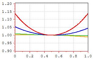
[file: D:\Lab documentation\5117.-109 Streak camera\Anomaly correction measurements\2016-02-25 LED TB1-4\Analysis\timebase1-4.txt]
To compare them, the time-axis (x-axis) is normalized to 1. Basically, only timebase 3 and 4 deviate significantly.
In the following graph, the ‘sensitivity’ deviation is show for 4 single sweep timebases. (5ns : red, 10 ns : green, 20 ns : blue, 50 ns : orange) (using a 2nd degree polynomial fit)
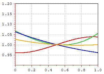
[file: D:\Lab documentation\5117.-109 Streak camera\Anomaly correction measurements\2016-03-01 LED SingleSweep\Analysis\SingleSweep 5-50ns sensitivities compared.txt]
The error in the green and blue curve is estimated to be 10%; So if needed, a better measurement has to be done.
Streak camera image tilt/shift
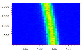
Using Synchroscan timebase 4, also the calibration lamp was used as a CW light source (2nd image is the line at 425 nm)
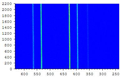
[ file: D:\Lab documentation\5117.-109 Streak camera\Anomaly correction measurements\2016-02-24 Calibration lamp TB4\3.img ]
The lines seem to be sligthtly tilted or shifted. One explanation might be that the CCD camera to record the image is slightly rotated. The positions of the maximum of the line at 425 nm were determined as a function of time :
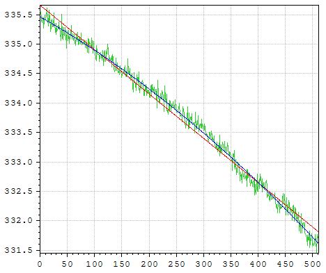
[ file: D:\Lab documentation\5117.-109 Streak camera\Anomaly correction measurements\2016-02-24 Calibration lamp TB4\Analysis\Positions img3 425 nm as pixelnrs .txt ]
The x-axis is now the array-element number along the time axis. The y-axis is the array-element number along the frequency axis.
The green line is the position of the maxima. . It is not a flat line, as it should be.
The red line is a fit with a 1st degree polynomial, the blue line a 2nd degree polynomial.
The fact that a 2nd degree polynomial fits clearly better, seems to rule out the explanation that the CCD camera is simply rotated.
But, as a first order approximation (using the 1st degree polynomial), one could assume the image IS rotated, and then correct it, by rotating the image by -0.432 degree CCW from the x-axis (see MatrixCalc, tab ‘Streak’, ‘Rotate (deg)’).
2. Using the same method to fit the LED data of SynchroScan Timebase 1-4 with 2 gaussians yields :
| Time base | Angle |
| 1 | -0.433 |
| 2 | -0.411 |
| 3 | -0.409 |
| 4 | -0.416 |
(average angle = -0.417)
NB: for all 4 datas : a 2nd degree polynomial fits better !
Using the same method to fit the LED data of SingleSweep 5-50nswith 2 gaussians yields :
| Time base | Angle |
| 5 ns | -0.428 |
| 10 ns | -0.585 |
| 20 ns | -0.464 |
| 50 ns | -0.473 |
| 50 ns B | -0.418 |
| 50 ns C | -0.397 |
NB: for all datas : a 2nd degree polynomial fits better !
It might be that it’s not the CCD camera which is slightly rotated, but e.g. the sweep electrodes are slightly non-uniform, so the electrons are not swept perfectly vertical (in time), but slightly deviated.